In this tutorial, we try and find the optimal racing line for a selection of AWS DeepRacer tracks. The AWS DeepRacer program consists of a physical 1/18th-scale model car with mounted camera, a platform to train these model cars to self-drive on virtual tracks and a league that races on physical tracks. The primary reason for not training directly on AWS is the opaque nature of its training process, which limits our ability to understand the underlying mechanism.

Our approach involves training a reinforcement learning agent in a car racing environment to achieve fast lap times, which we then transfer to the AWS DeepRacer tracks. To accomplish this task, we’ll be leveraging a couple of key tools:

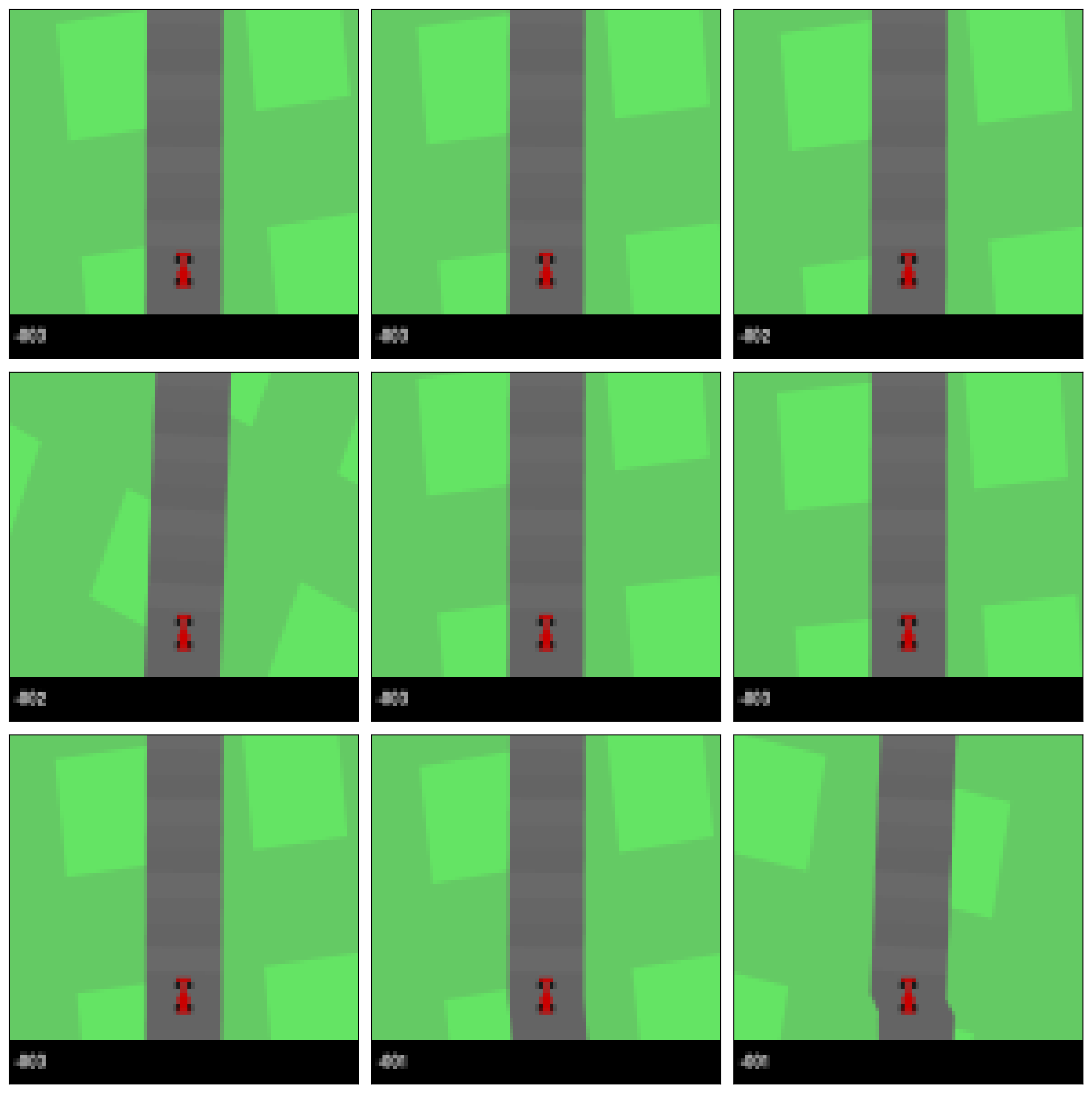
We’ll utilize the CarRacing environment from Gymnasium¹, a suite of reinforcement learning environments, forked from the unmaintained OpenAI Gym². The CarRacing environment models the vehicle as a powerful rear-wheel drive car and offers a realistic representation of car dynamics and track conditions, including ABS sensors and friction detectors. The environment provides both continuous and discrete action spaces, represents the race state as a zoomed-in, top-down color image and has a built-in reward function that rewards track tiles visited and penalises passing time. To simplify the model, we’ll be using the discrete action space, which has 5 actions: do nothing (0), steer left (1), steer right(2), apply gas (3), and apply brakes (4).
For the machine learning model, we will employ the Proximal Policy Optimization (PPO) algorithm³ implemented in Stable Baselines3 (SB3)⁴. PPO is a robust reinforcement learning algorithm from OpenAI and is one of two algorithms available for model training on AWS DeepRacer, alongside Soft Actor-Critic (SAC). We have chosen PPO for our project due to its compatibility with discrete space operations.

vec_env = make_vec_env(lambda: gym.make("CarRacing-v2"), n_envs=9)
obs = vec_env.reset()

for _ in range(100):  # skip the initial zooming-in animation
    obs, _, _, _ = vec_env.step(np.zeros((9, 3)))  # do nothing

fig, ax = plt.subplots(3, 3, figsize=(12, 12))
for i, row in enumerate(ax):
    for j, col in enumerate(row):
        col.imshow(obs[3 * i + j])
        col.set_xticks([])
        col.set_yticks([])
plt.tight_layout()

plt.show()

png

Training an Agent for the CarRacing Environment

To make things easier for the agent, the environment undergoes several modifications through a number of wrappers:

FrameSkip: implements frame skipping by returning only every n-th frame. It significantly speeds up the training process by reducing the frequency of frame updates that the agent needs to process. During the skipped frames, the same action is repeated, and the rewards are accumulated, ensuring that the reward signal is consistent despite the reduced frame rate.
ResizeObservation: resizes the observation space of the environment, typically making it smaller to reduce the complexity of the input that the agent has to process. For our task, it resizes the observations to 64 × 64 resolution, simplifying the visual input for the agent.
GrayScaleObservation: converts the observation space from color (RGB) to grayscale. By reducing the color dimensions, it simplifies the observation space, which can reduce the computational requirements as the agent has fewer visual features to process.

Then we batch up 9 environments and apply a few additional wrappers to the vectorised environment:

VecFrameStack: stacks multiple consecutive frames together and provides them as a single observation. This is particularly useful in environments where understanding the temporal dynamics is important, as it gives the agent access to a sequence of past frames. This temporal context can significantly enhance the agent’s ability to make informed decisions based on the observed motion patterns or changes over time.
VecNormalize: normalizes the environment’s rewards (and optionally the observations). Normalizing rewards can stabilize the training process by keeping the reward scale consistent across different environments or episodes. It’s particularly useful when dealing with environments that have varying reward scales or when combining multiple environments, as it ensures that the agent’s learning process is not biased towards environments with inherently higher or more variable rewards.

class FrameSkip(gym.Wrapper):
    """
    Return only every ``skip``-th frame (frameskipping).
    :param env: the environment
    :param skip: number of ``skip``-th frame
    """

    def __init__(self, env, skip=4):
        super().__init__(env)
        self._skip = skip

    def step(self, action):
        """
        Step the environment with the given action. Repeat action, sum reward.
        :param action: the action
        :return: observation, reward, terminated, truncated, information
        """
        total_reward = 0.0
        for _ in range(self._skip):
            obs, reward, terminated, truncated, info = self.env.step(action)
            total_reward += float(reward)
            if terminated or truncated:
                break

        return obs, total_reward, terminated, truncated, info

from gymnasium.wrappers import GrayScaleObservation, ResizeObservation
from stable_baselines3.common.env_util import make_vec_env
from stable_baselines3.common.vec_env import DummyVecEnv, VecFrameStack, VecNormalize


def create_env(env_id="CarRacing-v2"):
    env = gym.make(env_id, render_mode="rgb_array", continuous=False)
    env = FrameSkip(env, skip=2)
    env = ResizeObservation(env, shape=64)
    env = GrayScaleObservation(env, keep_dim=True)
    return env

vec_env = make_vec_env(create_env, n_envs=9)
vec_env = VecFrameStack(vec_env, n_stack=4)
vec_env = VecNormalize(vec_env, norm_obs=False, norm_reward=True)

Next, we initialise the Proximal Policy Optimization (PPO) model using the Stable Baselines3 library. We use the recommended hyperparameters from the reinforcement learning training framework RL Baselines3 Zoo⁵ and train the model for a total of 2,000,000 timesteps over all the environments.

from stable_baselines3 import PPO


model = PPO(
    "MlpPolicy",
    vec_env,
    learning_rate=lambda remaining_progress: remaining_progress * 1e-4,
    n_steps=512,
    batch_size=128,
    policy_kwargs=dict(
        activation_fn=nn.GELU,
        net_arch=dict(pi=[256], vf=[256]),
        ortho_init=False,
    ),
    verbose=1,
)

model.learn(total_timesteps=2_000_000)
model.save("ppo_car_racing_discrete")

Note: this takes 8h30 to train on a Intel i7-8700K CPU and 2 × NVIDIA Quadro GP100

Results

Video

To view the results, we roll out a batch of 9 episodes using the trained model, capture the frames, and stitch them together to create a video.

import imageio


images = []
obs = model.env.reset()
for _ in range(1_000):
    image = model.env.render(mode="rgb_array")
    images.append(image)

    action, _ = model.predict(obs, deterministic=True)
    obs, _, _ ,_ = model.env.step(action)

    
imageio.mimsave('output.gif', images, format='GIF', fps=50)

Trajectories

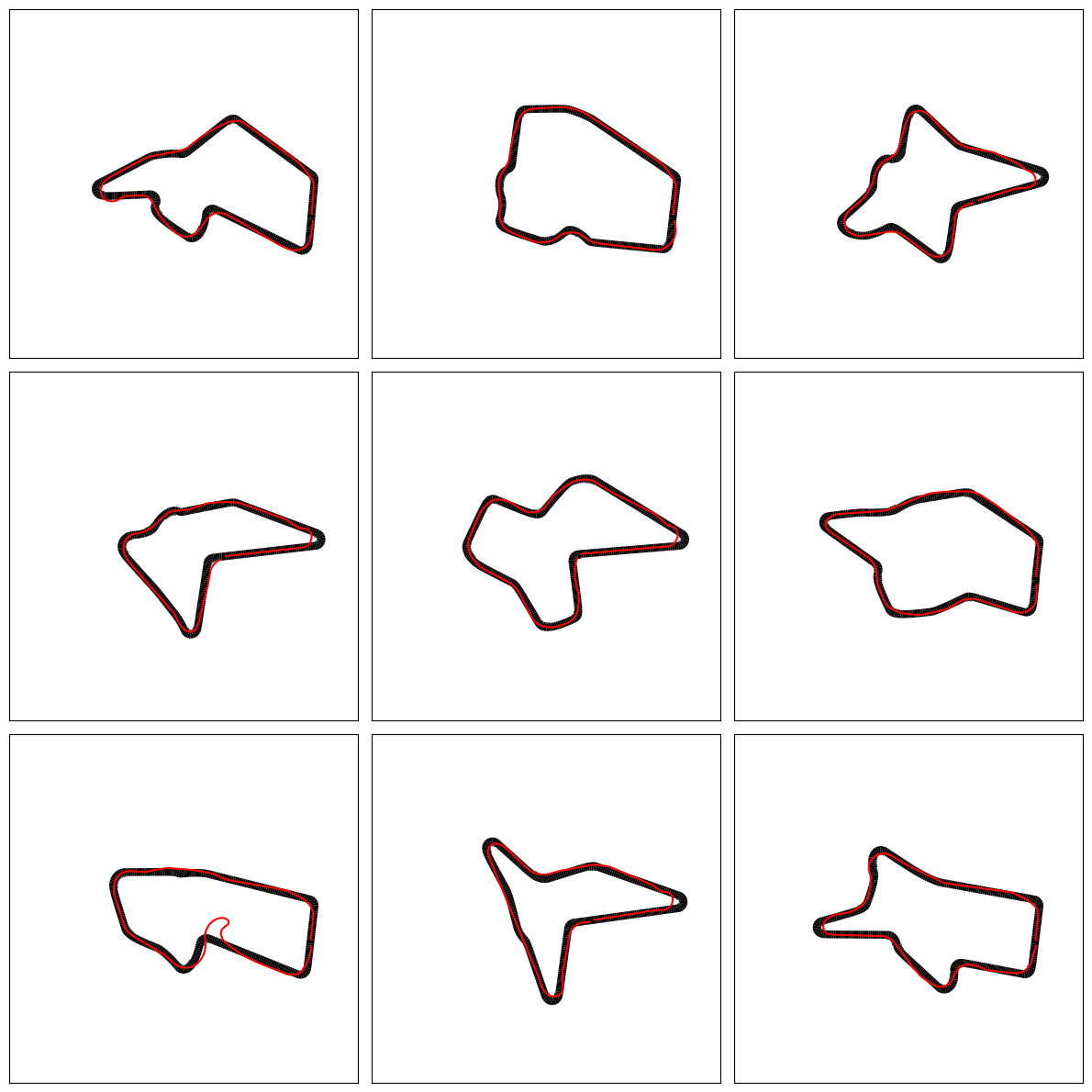
In order to visualise the car trajectories, we follow the trained model deterministically, record the cars’ positions at each step, for each of the nine parallel environment instances. Because we are dealing with environments in parallel, care must be taken to handle episode truncation as different episodes may terminate at different times.

import matplotlib.pyplot as plt
import numpy as np

from matplotlib.patches import Polygon
from scipy.spatial.distance import cdist
from tqdm import tqdm


obs = model.env.reset()
road_poly = [model.env.envs[i].get_wrapper_attr("road_poly") for i in range(9)]

positions = []
for _ in tqdm(range(499)):
    action, _ = model.predict(obs, deterministic=True)
    obs, _, _, _ = model.env.step(action)
    positions.append([list(env.car.hull.position) for env in model.env.envs])
    
positions = np.swapaxes(np.array(positions), 0, 1)

fig, ax = plt.subplots(3, 3, figsize=(12, 12))
for i, row in enumerate(ax):
    for j, col in enumerate(row):
        for poly, _ in road_poly[3 * i + j]:
            col.add_patch(Polygon(poly, facecolor="k"))

        # Truncate when within distance of 10 to starting point and after first 50 steps
        distance_from_start = cdist(positions[3 * i + j], positions[3 * i + j][[0]])
        index = next(i for i, d in enumerate(distance_from_start) if i > 50 and d < 10)

        x = positions[3 * i + j, :index, 0]
        y = positions[3 * i + j, :index, 1]
        col.plot(x, y, "-r")
        col.set_xlim([-300, 300])
        col.set_ylim([-300, 300])
        col.set_xticks([])
        col.set_yticks([])

plt.tight_layout()
plt.show()

png

AWS DeepRacer Tracks

With a trained model in hand, we can now turn to applying the model to AWS DeepRacer tracks. We need a way of loading the tracks, into the CarRacing environment. First, we download the track waypoint files⁶(https://github.com/aws-deepracer-community/deepracer-race-data/tree/main/raw_data/tracks), which each contain a NumPy array of shape (num_waypoints, 6), with the values in each row being: center_x, center_y, inside_x, inside_y, outside_x, outside_y. Then, we define a custom environment DeepRacerEnv, which inherits from the CarRacing class and override two methods to enable the CarRacing environment to process and interpret track data from AWS DeepRacer, which is stored in the .npy file format.

class DeepRacerEnv(CarRacing):
    def __init__(self, track_file, track_scale=25.0, track_width_scale=0.5, **kwargs):
        super().__init__(**kwargs)

        arr = np.load(track_file).reshape(-1, 3, 2) * track_scale

        # Scale track width
        arr[:, 1] = arr[:, 0] + track_width_scale * (arr[:, 1] - arr[:, 0])
        arr[:, 2] = arr[:, 0] + track_width_scale * (arr[:, 2] - arr[:, 0])

        self.track_waypoints = arr

        self.fd_tile = fixtureDef(
            shape=polygonShape(vertices=[(0, 0), (1, 0), (1, -1), (0, -1)])
        )

    def _create_track(self):
        """
        Creates the track by reading waypoints from the npy file.
        The track waypoints are expected to be in the format:
        (center_x, center_y, inside_x, inside_y, outside_x, outside_y).
        """
        self.road = []
        self.track = []
        self.road_poly = []

        for idx in range(len(self.track_waypoints) - 1):
            if np.array_equal(self.track_waypoints[idx], self.track_waypoints[idx + 1]):
                continue  # some waypoints are erroneously duplicated

            center_current, inside_current, outside_current = self.track_waypoints[idx]
            center_next, inside_next, outside_next = self.track_waypoints[idx + 1]

            vertices = [
                tuple(inside_current),
                tuple(outside_current),
                tuple(outside_next),
                tuple(inside_next),
            ]

            # Create the track segment
            self.fd_tile.shape.vertices = vertices
            t = self.world.CreateStaticBody(fixtures=self.fd_tile)
            t.userData = t
            t.color = self.road_color
            t.road_visited = False
            t.road_friction = 1.0
            t.idx = idx
            t.fixtures[0].sensor = True
            self.road.append(t)
            self.road_poly.append((vertices, t.color))

            # Calculate the angle for the track segment
            dx, dy = center_next - center_current
            angle = math.atan2(dy, dx) + np.pi / 2.0

            # Append information for self.track
            self.track.append((idx, angle, *center_current))
            
        return True

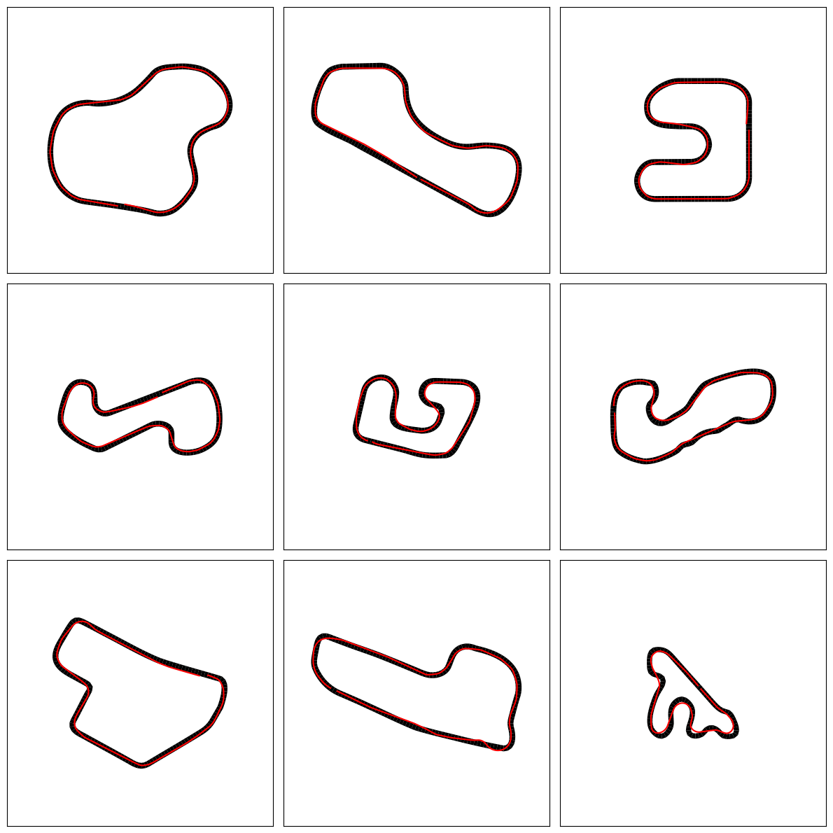
Following this, we will assemble the trajectories in the same as the previous section, except that we will explicitly load different tracks for each environment in the batch. Here we have chosen the monthly tracks from the open category of the 2022 AWS DeepRacer League.

def create_aws_deep_racer_env(track_id):
    env = DeepRacerEnv(track_id, render_mode="rgb_array", continuous=False)
    env = FrameSkip(env, skip=2)
    env = ResizeObservation(env, shape=64)
    env = GrayScaleObservation(env, keep_dim=True)
    return env


env_fns_open = [
    lambda: create_aws_deep_racer_env("../data/Tracks/2022_march_open.npy"),
    lambda: create_aws_deep_racer_env("../data/Tracks/2022_april_open.npy"),
    lambda: create_aws_deep_racer_env("../data/Tracks/2022_may_open.npy"),
    lambda: create_aws_deep_racer_env("../data/Tracks/2022_june_open.npy"),
    lambda: create_aws_deep_racer_env("../data/Tracks/2022_july_open.npy"),
    lambda: create_aws_deep_racer_env("../data/Tracks/2022_august_open.npy"),
    lambda: create_aws_deep_racer_env("../data/Tracks/2022_september_open.npy"),
    lambda: create_aws_deep_racer_env("../data/Tracks/2022_october_open.npy"),
    lambda: create_aws_deep_racer_env("../data/Tracks/2022_reinvent_champ.npy"),
]

vec_env = DummyVecEnv(env_fns_open)
vec_env = VecFrameStack(vec_env, n_stack=4)
vec_env = VecNormalize(vec_env, norm_obs=False, norm_reward=True)

obs = model.env.reset()
road_poly = [model.env.envs[i].get_wrapper_attr("road_poly") for i in range(9)]

positions = []
for _ in tqdm(range(1_500)):
    action, _ = model.predict(obs, deterministic=True)
    obs, _, done, _ = model.env.step(action)
    positions.append([list(env.car.hull.position) for env in model.env.envs])
    
positions = np.swapaxes(np.array(positions), 0, 1)

fig, ax = plt.subplots(3, 3, figsize=(12, 12))
for i, row in enumerate(ax):
    for j, col in enumerate(row):
        for poly, _ in road_poly[3 * i + j]:
            col.add_patch(Polygon(poly, facecolor="k"))
            
        # Truncate when within distance of 10 to starting point and after first 50 steps
        distance_from_start = cdist(positions[3 * i + j], positions[3 * i + j][[0]])
        index = next(i for i, d in enumerate(distance_from_start) if i > 50 and d < 10)
        x = positions[3 * i + j, :index, 0]
        y = positions[3 * i + j, :index, 1]
        col.plot(x, y, "-r")
        col.set_xlim([-300, 300])
        col.set_ylim([-300, 300])
        col.set_xticks([])
        col.set_yticks([])

plt.tight_layout()
plt.show()

png

Looking at the results on these held-out tracks, we can see that the agent performs quite well in certain cases, even driving on a racing line optimised for speed.

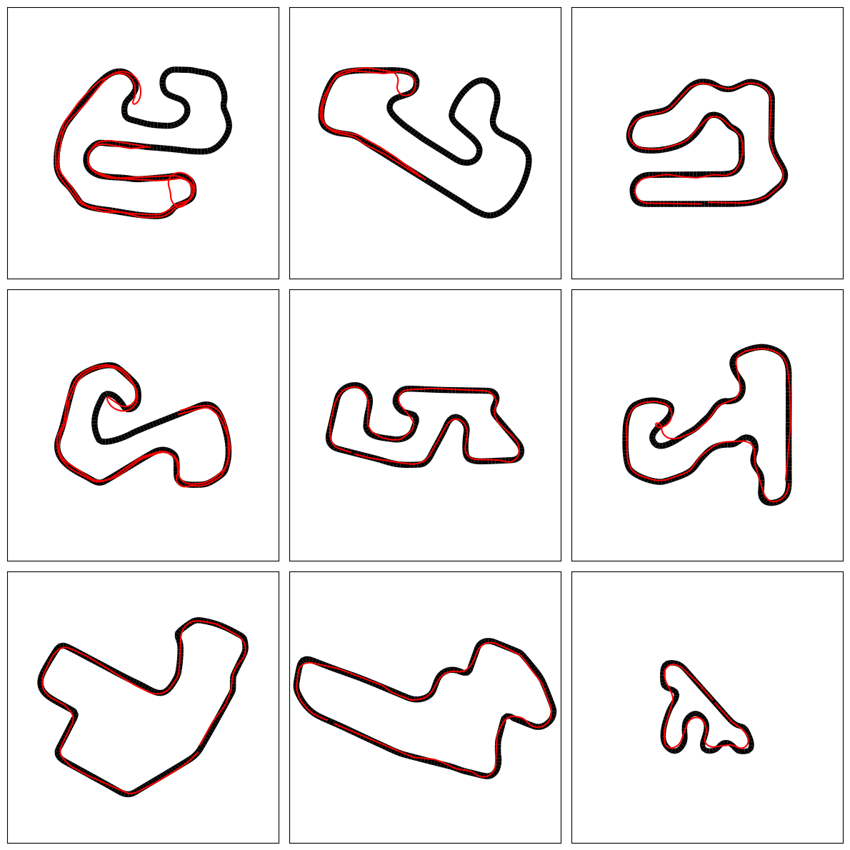
Now, we try our hand at the monthly tracks from the professional category of the 2022 AWS DeepRacer League. These follow the general shape of their counterparts in the open category, but feature more challenging twists and turns.

env_fns_pro = [
    lambda: create_aws_deep_racer_env("../data/Tracks/2022_march_pro.npy"),
    lambda: create_aws_deep_racer_env("../data/Tracks/2022_april_pro.npy"),
    lambda: create_aws_deep_racer_env("../data/Tracks/2022_may_pro.npy"),
    lambda: create_aws_deep_racer_env("../data/Tracks/2022_june_pro.npy"),
    lambda: create_aws_deep_racer_env("../data/Tracks/2022_july_pro.npy"),
    lambda: create_aws_deep_racer_env("../data/Tracks/2022_august_pro.npy"),
    lambda: create_aws_deep_racer_env("../data/Tracks/2022_september_pro.npy"),
    lambda: create_aws_deep_racer_env("../data/Tracks/2022_october_pro.npy"),
    lambda: create_aws_deep_racer_env("../data/Tracks/2022_reinvent_champ.npy"),
]

vec_env = DummyVecEnv(env_fns_pro)
vec_env = VecFrameStack(vec_env, n_stack=4)
vec_env = VecNormalize(vec_env, norm_obs=False, norm_reward=True)

obs = model.env.reset()
road_poly = [model.env.envs[i].get_wrapper_attr("road_poly") for i in range(9)]

positions = []
for _ in tqdm(range(1_500)):
    action, _ = model.predict(obs, deterministic=True)
    obs, _, done, _ = model.env.step(action)
    positions.append([list(env.car.hull.position) for env in model.env.envs])
    
positions = np.swapaxes(np.array(positions), 0, 1)

fig, ax = plt.subplots(3, 3, figsize=(12, 12))
for i, row in enumerate(ax):
    for j, col in enumerate(row):
        for poly, _ in road_poly[3 * i + j]:
            col.add_patch(Polygon(poly, facecolor="k"))
            
        # Truncate when within distance of 10 to starting point and after first 50 steps
        distance_from_start = cdist(positions[3 * i + j], positions[3 * i + j][[0]])
        index = next(i for i, d in enumerate(distance_from_start) if i > 50 and d < 10)
        x = positions[3 * i + j, :index, 0]
        y = positions[3 * i + j, :index, 1]
        col.plot(x, y, "-r")
        col.set_xlim([-300, 300])
        col.set_ylim([-300, 300])
        col.set_xticks([])
        col.set_yticks([])

plt.tight_layout()
plt.show()

png

The result is a mixed bag. The performance on some tracks is satisfactory, but in others, the car seems to do a U-turn. This may be because when travelling fast around sharp corners, the car is prone to spinning out, and since it only relies on image input, resumes driving in whatever direction it’s facing.

Adapting Gymnasium to Find DeepRacer Racing Lines

Train a PPO agent from Stable Baselines3 to master the Gymnasium CarRacing environment.

Training an Agent for the CarRacing Environment

Results

Video

Trajectories

AWS DeepRacer Tracks

References

-
Towers, M., Terry, J. K., Kwiatkowski, A., Balis, J. U., de Cola, G., Deleu, T., Goulão, M., Kallinteris, A., KG, A., Krimmel, M., Perez-Vicente, R., Pierré, A., Schulhoff, S., Tai, J. J., Tan, A. J. S., & Younis, O. G. (2023). Gymnasium. Computer software. ↩︎
Brockman, G., Cheung, V., Pettersson, L., Schneider, J., Schulman, J., Tang, J., & Zaremba, W. (2016). OpenAI Gym. Computer software. ↩︎
Schulman, J., Wolski, F., Dhariwal, P., Radford, A., & Klimov, O. (2017). Proximal Policy Optimization Algorithms. OpenAI. ↩︎
Raffin, A., Hill, A., Gleave, A., Kanervisto, A., Ernestus, M., & Dormann, N. (2021). Stable-Baselines3: Reliable Reinforcement Learning Implementations. Computer Software. ↩︎
AWS DeepRacer Community Race Data Repository. (2023). Computer software. ↩︎
Timothy Leung