In this tutorial, we’ll be building a transformer-based model for Handwritten Mathematical Expression Recognition (HMER). While the output of the model is LaTeX text, the input is a set of images rendered from stroke data making this an offline task. The online variation of this task would see us directly using the stroke data, which in addition to coordinates, can include useful attributes like pen pressure and timestamp data.

Although this task dates back to the 1960s, the first Competition on Recognition of Online Handwritten Mathematical Expressions (CROHME) was held at the International Conference on Document Analysis and Recognition (ICDAR) in 2011. Since then it has been run many times, most recently in 2023. We’ll be using the CROHME 2023 dataset¹ to train this model.

Tokenization

Tokenization is an important first step in making the LaTeX text interpretable by a Machine Learning model. Instead of using Hugging Face Tokenizers², a powerful library that includes tokenization algorithms such as Byte-Pair Encoding (BPE) and WordPiece, we’ll build our own basic tokeniser, LaTeXTokenizer, from scratch so that we can peer into how tokenization, vocabulary building, and encoding/decoding work.

import collections
import re

from typing import Dict, List, Tuple, Union


class LaTeXTokenizer:
    def __init__(self):
        self.special_tokens = ["[PAD]", "[BOS]", "[EOS]", "[UNK]"]
        self.vocab = {}
        self.token_to_id = {}
        self.id_to_token = {}

    def tokenize(self, text: str) -> List[str]:
        # Tokenize LaTeX using regex to capture commands, numbers and other characters
        return re.findall(r"\\[a-zA-Z]+|\\.|[a-zA-Z0-9]|\S", text)

    def build_vocab(self, texts: List[str]):
        # Add special tokens to vocabulary
        for token in self.special_tokens:
            self.vocab[token] = len(self.vocab)

        # Create a counter to hold token frequencies
        counter = collections.Counter()

        # Tokenize each text and update the counter
        for text in texts:
            tokens = self.tokenize(text)
            counter.update(tokens)

        # Add tokens to vocab based on their frequency
        for token, _ in counter.most_common():
            if token not in self.vocab:
                self.vocab[token] = len(self.vocab)

        # Build dictionaries for token to ID and ID to token conversion
        self.token_to_id = self.vocab
        self.id_to_token = {v: k for k, v in self.vocab.items()}

    def encode(self, text: str) -> List[int]:
        # Tokenize the input text and add start and end tokens
        tokens = ["[BOS]"] + self.tokenize(text) + ["[EOS]"]

        # Map tokens to their IDs, using [UNK] for unknown tokens
        unk_id = self.token_to_id["[UNK]"]
        return [self.token_to_id.get(token, unk_id) for token in tokens]

    def decode(self, token_ids: List[int]) -> List[str]:
        # Map token IDs back to tokens
        tokens = [self.id_to_token.get(id, "[UNK]") for id in token_ids]

        # Remove tokens beyond the [EOS] token
        if "[EOS]" in tokens:
            tokens = tokens[: tokens.index("[EOS]")]

        # Replace [UNK] with ?
        tokens = ["?" if token == "[UNK]" else token for token in tokens]

        # Reconstruct the original text, ignoring special tokens
        return "".join([token for token in tokens if token not in self.special_tokens])

I’d like to highlight several interesting aspects of the LaTeXTokenizer code:

we designate 4 special tokens that aid us in various downstream tasks: a padding token [PAD], a beginning of sentence token [BOS], an end of sentence token [EOS] and an unknown token [UNK]
we use the regular expression \\[a-zA-Z]+|\\.|[a-zA-Z0-9]|\S to capture LaTeX commands, numbers, and other characters
decoded LaTeX strings are truncated upon encountering an [EOS] token
encoded tokens are prefixed by the [BOS] token and suffixed with the [EOS] token
encoded tokens that are not in the vocabulary are designed [UNK], meaning that they weren’t seen during training and are only seen during val/test/predict time

Let’s have a look at the LaTeXTokenizer class in action.

Vocabulary Building

First, let’s instantiate the LaTeXTokenizer class and build the vocabulary with two example mathematical expressions written in LaTeX: $a^2 + b^2 = c^2$ and $e^{i\pi} + 1 = 0$.

tokenizer = LaTeXTokenizer()
tokenizer.build_vocab(["a^2 + b^2 = c^2", "e^{i\\pi} + 1 = 0"])

After running this code snippet, you can inspect the vocabulary to see the tokens and their corresponding IDs.

print(tokenizer.vocab)

{'[PAD]': 0, '[BOS]': 1, '[EOS]': 2, '[UNK]': 3, '^': 4, '2': 5, '+': 6, '=': 7, 'a': 8, 'b': 9, 'c': 10, 'e': 11, '{': 12, 'i': 13, '\\pi': 14, '}': 15, '1': 16, '0': 17}

Notice that the special tokens [PAD], [BOS], [EOS] and [UNK] are also present in the vocabulary.

Encoding

Now let’s encode a new mathematical expression, $i^2 = -1$, into its corresponding token IDs. The encode method will tokenize the input string and convert each token into its respective ID from the vocabulary. Unknown tokens, if any, will be mapped to [UNK].

ids = tokenizer.encode('i^2 = -1')
print(ids)

[1, 13, 4, 5, 7, 3, 16, 2]

Decoding

Finally, to check that the encoding makes sense, we decode the token IDs back into a LaTeX string. The decode method will convert the token IDs back to their original LaTeX tokens, joining them into a LaTeX expression.

latex = tokenizer.decode(ids)
print(latex)

i^2=?1

Notice that the minus symbol (-) was not present in the vocabulary and so was encoded into [UNK], represented in the decoded string as a ?.

CROHME Dataset

The CROHME dataset is a collection of handwritten mathematical expressions with their corresponding LaTeX annotations. In this section, we’ll be parsing the dataset’s InkML files and preparing them for model training.

InkML is a data format for representing digital ink entered with an electronic pen. It supports many attributes including writer information (like age, gender, and handedness), pen pressure, pen tilt, stroke data, and ground truth data. For our purpose, we’ll only be using the stroke data and ground truth LaTeX string, which we parse using the parse_inkml function. Instead of rendering the stroke data and extracting the LaTeX string on-the-fly, as data gets loaded into the model, we cache them to the filesystem to speed things up.

import io
import matplotlib.pyplot as plt
import xml.etree.ElementTree as ET

from pathlib import Path
from PIL import Image


def parse_inkml(inkml_file_path, ns={"inkml": "http://www.w3.org/2003/InkML"}):
    tree = ET.parse(inkml_file_path)
    root = tree.getroot()

    strokes = []
    for trace in root.findall(".//inkml:trace", ns):
        coords = trace.text.strip().split(",")
        coords = [
            (float(x), -float(y))  # Invert y-axis to match InkML's coordinate system
            for x, y, *z in [coord.split() for coord in coords]
        ]
        strokes.append(coords)

    latex = root.find('.//inkml:annotation[@type="truth"]', ns).text.strip(" $")

    return strokes, latex


def cache_data():
    fig, ax = plt.subplots()

    for inkml_file in data_dir.glob("*/*.inkml"):
        img_file = inkml_file.with_suffix(".png")
        txt_file = inkml_file.with_suffix(".txt")

        strokes, latex = parse_inkml(inkml_file)

        # Write LaTeX to file
        with open(txt_file, "w") as f:
            f.write(latex)

        # Render strokes to file
        ax.set_axis_off()
        ax.set_aspect("equal")
        for coords in strokes:
            x, y = zip(*coords)
            ax.plot(x, y, color="black", linewidth=2)
        buf = io.BytesIO()
        plt.savefig(buf, bbox_inches="tight", pad_inches=0)
        plt.cla()
        buf.seek(0)
        img = Image.open(buf).convert("RGB")
        img.save(img_file)


cache_data()

Next, we wrap CROHMEDataset around this cached image and LaTeX data, storing the corresponding train/val splits in a CROHMEDataModule. The collate_fn method takes care of centering and padding images within a fixed size canvas as well as padding token sequences to the maximum length of the batch. The images are randomly distorted using RandomPerspective to make the model more robust.

import lightning.pytorch as pl
import torch
import torch.nn.functional as F

from pathlib import Path
from PIL import Image
from torch import nn, optim, Tensor
from torch.nn.utils.rnn import pad_sequence
from torch.utils import data
from torchvision import transforms


class CROHMEDataset(data.Dataset):
    def __init__(self, latex_files, tokenizer, transform):
        super().__init__()
        self.latex_files = list(latex_files)
        self.tokenizer = tokenizer
        self.transform = transform

    def __len__(self):
        return len(self.latex_files)

    def __getitem__(self, idx):
        latex_file = self.latex_files[idx]
        image_file = latex_file.with_suffix(".png")

        with open(latex_file) as f:
            latex = f.read()

        x = self.transform(Image.open(image_file))
        y = Tensor(self.tokenizer.encode(latex))
        return x, y


class CROHMEDataModule(pl.LightningDataModule):
    def __init__(
        self,
        data_dir: str,
        batch_size: int = 1,
        num_workers: int = 0,
        pin_memory: bool = False,
    ):
        super().__init__()
        self.save_hyperparameters()
        self.data_dir = Path(data_dir)
        self.transform = transforms.Compose(
            [
                transforms.RandomPerspective(distortion_scale=0.1, p=0.5, fill=255),
                transforms.ToTensor(),
            ]
        )

    def setup(self, stage):
        latexes = []
        for latex_file in self.data_dir.glob("train/*.txt"):
            with open(latex_file) as f:
                latexes.append(f.read())

        self.tokenizer = LaTeXTokenizer()
        self.tokenizer.build_vocab(latexes)
        self.vocab_size = len(self.tokenizer.vocab)

        if stage == "fit" or stage is None:
            self.train_dataset = CROHMEDataset(
                self.data_dir.glob("train/*.txt"), self.tokenizer, self.transform
            )
            self.val_dataset = CROHMEDataset(
                self.data_dir.glob("val/*.txt"), self.tokenizer, self.transform
            )

    def collate_fn(self, batch, max_width: int = 512, max_height: int = 384):
        images, labels = zip(*batch)

        # Create a white background for each image in the batch
        src = torch.ones((len(images), 3, max_height, max_width))

        # Center and pad individual images to fit into the white background
        for i, img in enumerate(images):
            height_start = (max_height - img.size(1)) // 2
            height_end = height_start + img.size(1)
            width_start = (max_width - img.size(2)) // 2
            width_end = width_start + img.size(2)
            src[i, :, height_start:height_end, width_start:width_end] = img

        # Pad sequences for labels and create attention mask
        tgt = pad_sequence(labels, batch_first=True).long()
        seq_len = tgt.size(1)
        tgt_mask = torch.triu(torch.ones(seq_len, seq_len) * float("-inf"), diagonal=1)

        return src, tgt, tgt_mask

    def train_dataloader(self):
        return data.DataLoader(
            self.train_dataset,
            batch_size=self.hparams.batch_size,
            num_workers=self.hparams.num_workers,
            collate_fn=self.collate_fn,
            pin_memory=self.hparams.pin_memory,
        )

    def val_dataloader(self):
        return data.DataLoader(
            self.val_dataset,
            batch_size=self.hparams.batch_size,
            num_workers=self.hparams.num_workers,
            collate_fn=self.collate_fn,
            pin_memory=self.hparams.pin_memory,
        )

Visualising a Batch of Data

Let’s inspect a batch of data to see what’s being fed to the model.

datamodule = CROHMEDataModule("../data/CROHME/", batch_size=16)
datamodule.setup(stage="fit")

tokenizer = datamodule.tokenizer

train_dataloader = datamodule.train_dataloader()
batch = next(iter(train_dataloader))
src, tgt, tgt_mask = batch

Here,

src contains the images of the handwritten mathematical expressions;
tgt contains the token IDs representing the LaTeX expressions; and
tgt_mask is the attention mask, which we’ll explain later on.

Handwritten Image

from torchvision.utils import make_grid

plt.imshow(make_grid(src, nrow=4).permute(1, 2, 0))
plt.axis("off")

(-0.5, 2057.5, 1545.5, -0.5)

png

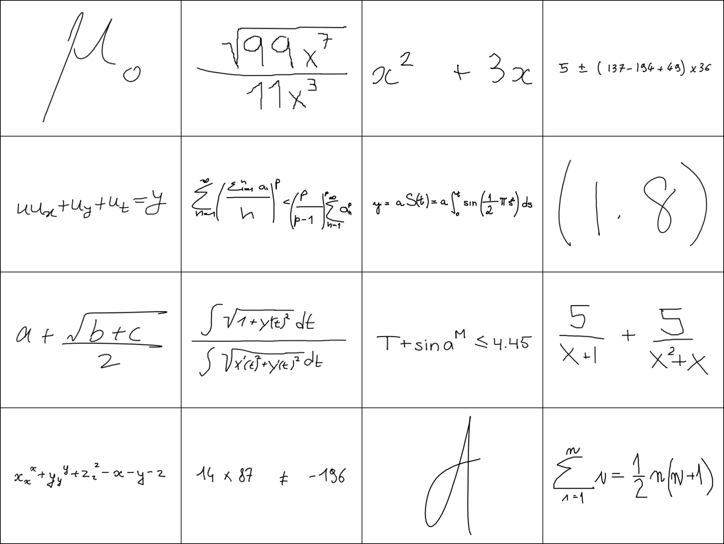
LaTeX String

for t in tgt:
    print(tokenizer.decode(t.tolist()))

{\mu}_{o}
\frac{\sqrt{99{x^{7}}}}{11{x^{3}}}
x^2+3x
5\pm(137-194+49)\times36
uu_{x}+u_{y}+u_{t}=y
\sum_{n=1}^{\infty}{(\frac{\sum_{i=1}^{n}a_{i}}{n})^{p}}\lt{(\frac{p}{p-1})^{p}}\sum_{n=1}^{\infty}{a_{n}^{p}}
y=aS(t)=a\int_0^{t}\sin(\frac{1}{2}\pis^2)ds
\left(1.8\right)
a+\frac{\sqrt{b+c}}{2}
\frac{\int\sqrt{1+{y^{'}(t)^{2}}}dt}{\int\sqrt{{x^{'}(t)^{2}}+{y^{'}(t)^{2}}}dt}
{{T+\sin{a}^{M}}\leq4.45}
\frac{5}{x+1}+\frac{5}{{x^{2}}+x}
x_x^x+y_y^y+z_z^z-x-y-z
14\times87\neq-196
\mbox{d}
\sum_{i=1}^{n}i=\frac{1}{2}n(n+1)

Positional Encoding for Attention Models

In models like Transformers, positional information is not naturally captured by the self-attention mechanism. For this reason, we use a technique called positional encoding to give the model information about the relative positions of the tokens. Ensuring that the model can take into account the order of the tokens allows it to significantly improve its performance on sequence-based tasks.

We’ll be using two types of positional encodings: 1D and 2D positional encodings, which are essential for 1D sequences like text and 2D structures like images, respectively.

In the 1D case, each position in the sequence is encoded into a high-dimensional vector. We use sine and cosine functions of different frequencies to encode the positional information.
When dealing with images or any 2D data, a 2D positional encoding is more appropriate. Here, we use a similar technique but extend it to 2D. We calculate 1D positional encoding first and then use the outer product to construct the 2D positional encoding. This way, each position in a 2D structure (like an image) gets a unique encoding based on its row and column.

import math
import matplotlib.pyplot as plt


class PositionalEncoding1D(nn.Module):
    def __init__(
        self,
        d_model: int,
        dropout: float = 0.1,
        max_len: int = 1000,
        temperature: float = 10000.0,
    ):
        super().__init__()

        # Generate position and dimension tensors for encoding
        position = torch.arange(max_len).unsqueeze(1)
        dim_t = torch.arange(0, d_model, 2)
        div_term = torch.exp(dim_t * (-math.log(temperature) / d_model))

        # Initialize and fill the positional encoding matrix with sine/cosine values
        pe = torch.zeros(max_len, d_model)
        pe[:, 0::2] = torch.sin(position * div_term)
        pe[:, 1::2] = torch.cos(position * div_term)

        self.dropout = nn.Dropout(dropout)
        self.register_buffer("pe", pe)

    def forward(self, x):
        batch, sequence_length, d_model = x.shape
        return self.dropout(x + self.pe[None, :sequence_length, :])


class PositionalEncoding2D(nn.Module):
    def __init__(
        self,
        d_model: int,
        dropout: float = 0.1,
        max_len: int = 30,
        temperature: float = 10000.0,
    ):
        super().__init__()

        # Generate position and dimension tensors for 1D encoding
        position = torch.arange(max_len).unsqueeze(1)
        dim_t = torch.arange(0, d_model, 2)
        div_term = torch.exp(dim_t * (-math.log(temperature) / d_model))

        # Initialize and fill the 1D positional encoding matrix with sine/cosine values
        pe_1D = torch.zeros(max_len, d_model)
        pe_1D[:, 0::2] = torch.sin(position * div_term)
        pe_1D[:, 1::2] = torch.cos(position * div_term)

        # Compute the 2D positional encoding matrix using outer product
        pe_2D = torch.zeros(max_len, max_len, d_model)
        for i in range(d_model):
            pe_2D[:, :, i] = pe_1D[:, i].unsqueeze(-1) + pe_1D[:, i].unsqueeze(0)

        self.dropout = nn.Dropout(dropout)
        self.register_buffer("pe", pe_2D)

    def forward(self, x):
        batch, height, width, d_model = x.shape
        return self.dropout(x + self.pe[None, :height, :width, :])

Visualising Positional Encodings with Python

Understanding positional encodings can become much clearer when you visualise them.

1D Positional Encoding

First, we will create a 1D positional encoding with a d_model of 256 and a maximum length of 100. We will then use matshow from Matplotlib to display it as a heatmap that reflects the values of the positional encoding. The x-axis represents the dimension (d_model) and the y-axis represents the sequence length (up to max_len).

2D Positional Encoding

For the 2D positional encoding, we use a more complex visualisation. We create a 2D positional encoding with d_model set to 32 and max_len to 64. Each subplot below show different layers (or dimensions) of the 2D positional encoding, allowing you to see how each dimension encodes 2D positional information differently.

Transformer-based Model

While a range of architectures are suitable for sequence-based tasks, the Transformer-approach is particularly versatile. In our case, the image is encoded into a set of features, which is then decoded autoregressively.

Encoder: The encoder is based on the DenseNet121 architecture. Since DenseNet was trained to output the 1,000 ImageNet classes, we swap the final classifier layer with a 1×1 convolution to reduce the output to d_model dimensions. We add the 2D positional encodings before flattening it into a sequence to be consumed by the decoder.
Decoder: The decoder is a stack of transformer layers that takes both the source features from the encoder and the target text. The target text is embedded into d_model-dimensional vectors and augmented with 1D positional encodings. After that, the source features and target embeddings are processed through the transformer decoder stack to generate the output. The last fully connected layer (fc_out) maps the output of the transformer to the vocabulary size, effectively determining the next token’s likelihood in the sequence.

Training

During training, the encoder’s output features and a shifted copy of the target sequence are fed into the decoder. The model’s predictions are then compared to the actual target sequence to compute the loss, which is then backpropagated to update the model parameters.

As mentioned above, the attention mask is one of the inputs to the model, along with the handwritten image and the LaTeX. In autoregressive decoding, its purpose is to ensure that each token is predicted based only on previously generated tokens as well as the encoded representation. In the example attention mask below, cells shaded white are what we are allowed to see, while cells shaded grey are hidden. To predict the 0-th target token {, we are only allowed to see the [BOS] token. Jumping to the 6-th row, to predict the 6-th target token }, we are only allowed to see the token sequence [BOS], {, \mu, }, _, {, o.

Inference

During inference, we can use either greedy search or beam search to generate sequences. In both methods, the initial step starts with feeding the encoder’s output features into the decoder, followed by iterative steps to generate each subsequent token.

Greedy Search: In greedy decoding, the model chooses the most likely (highest probability) next step at each step in the sequence. This is computationally less expensive but may not always produce the most optimal sequences. During inference, we start with a [BOS] token and keep appending the token with the highest probability to the target sequence until it reaches max_seq_len or a [EOS] token is encountered.
Beam Search: Beam search keeps track of the top k (beam width) probable sequences at each step, expanding all of them at each step and keeping only the best k. This is computationally more expensive but usually produces better results. During inference, we start with a [BOS] token and and maintain multiple sequences for each item in the batch, updating them at each step based on their total log probability so far. Again, candidate sequences are stopped when [EOS] tokens are encountered and their scores frozen.

from torchvision.models import densenet121, DenseNet121_Weights


class Permute(nn.Module):
    def __init__(self, *dims: int):
        super().__init__()
        self.dims = dims

    def forward(self, x):
        return x.permute(*self.dims)


class Model(pl.LightningModule):
    def __init__(
        self,
        vocab_size: int,
        d_model: int,
        nhead: int,
        dim_feedforward: int,
        dropout: float,
        num_layers: int,
        lr: float = 1e-4,
    ):
        super().__init__()
        self.save_hyperparameters()
        self.example_input_array = (
            torch.rand(16, 3, 384, 512),  # batch x channel x height x width
            torch.ones(16, 64, dtype=torch.long),  # batch x sequence length
            torch.zeros(64, 64),  # sequence length x sequence length
        )

        # Define the encoder architecture
        densenet = densenet121(weights=DenseNet121_Weights.DEFAULT)
        self.encoder = nn.Sequential(
            nn.Sequential(*list(densenet.children())[:-1]),  # remove the final layer
            nn.Conv2d(1024, d_model, kernel_size=1),
            Permute(0, 2, 3, 1),
            PositionalEncoding2D(d_model, dropout),
            nn.Flatten(1, 2),
        )

        # Define the decoder architecture
        self.tgt_embedding = nn.Embedding(vocab_size, d_model, padding_idx=0)
        self.word_positional_encoding = PositionalEncoding1D(d_model, dropout)
        self.transformer_decoder = nn.TransformerDecoder(
            nn.TransformerDecoderLayer(
                d_model, nhead, dim_feedforward, dropout, batch_first=True
            ),
            num_layers,
        )
        self.fc_out = nn.Linear(d_model, vocab_size)

    def decoder(self, features, tgt, tgt_mask):
        padding_mask = tgt.eq(0)
        tgt = self.tgt_embedding(tgt) * math.sqrt(self.hparams.d_model)
        tgt = self.word_positional_encoding(tgt)
        tgt = self.transformer_decoder(
            tgt, features, tgt_mask=tgt_mask, tgt_key_padding_mask=padding_mask
        )
        output = self.fc_out(tgt)
        return output

    def forward(self, src, tgt, tgt_mask):
        features = self.encoder(src)
        output = self.decoder(features, tgt, tgt_mask)
        return output

    def training_step(self, batch, batch_idx):
        loss = self._shared_eval_step(batch, batch_idx)
        self.log(
            "train_loss",
            loss,
            on_step=True,
            on_epoch=True,
            sync_dist=True,
            prog_bar=True,
        )
        return loss

    def validation_step(self, batch, batch_idx):
        loss = self._shared_eval_step(batch, batch_idx)
        metrics = {"val_loss": loss}
        self.log_dict(metrics, sync_dist=True)
        return metrics

    def _shared_eval_step(self, batch, batch_idx):
        src, tgt, tgt_mask = batch
        tgt_in = tgt[:, :-1]
        tgt_out = tgt[:, 1:]
        output = self(src, tgt_in, tgt_mask[:-1, :-1])
        loss = F.cross_entropy(
            output.reshape(-1, self.hparams.vocab_size),
            tgt_out.reshape(-1),
            ignore_index=0,
        )
        return loss

    def beam_search(
        self,
        src,
        tokenizer,
        max_seq_len: int = 256,
        beam_width: int = 3,
    ) -> List[str]:
        with torch.no_grad():
            batch_size = src.size(0)
            vocab_size = self.hparams.vocab_size
            features = self.encoder(src).detach()
            features_rep = features.repeat_interleave(beam_width, dim=0)
            tgt_mask = torch.triu(
                torch.ones(max_seq_len, max_seq_len) * float("-inf"), diagonal=1
            ).to(src.device)

            # Initialize with [BOS]
            beams = torch.ones(batch_size, 1, 1).long().to(src.device)

            # Handle first step separately
            output = self.decoder(features, beams[:, 0, :], tgt_mask[:1, :1])
            next_probs = output[:, -1, :].log_softmax(dim=-1)
            beam_scores, indices = next_probs.topk(beam_width, dim=-1)
            beams = torch.cat(
                [beams.repeat_interleave(beam_width, dim=1), indices.unsqueeze(2)],
                dim=-1,
            )

            for i in range(2, max_seq_len):
                tgt = beams.view(batch_size * beam_width, i)
                output = self.decoder(features_rep, tgt, tgt_mask[:i, :i])
                next_probs = output[:, -1, :].log_softmax(dim=-1)

                next_probs += beam_scores.view(batch_size * beam_width, 1)
                next_probs = next_probs.view(batch_size, -1)

                beam_scores, indices = next_probs.topk(beam_width, dim=-1)
                beams = torch.cat(
                    [
                        beams[
                            torch.arange(batch_size).unsqueeze(-1),
                            indices // vocab_size,
                        ],
                        (indices % vocab_size).unsqueeze(2),
                    ],
                    dim=-1,
                )

        best_beams = beams[:, 0, :]  # taking the best beam for each batch
        return [tokenizer.decode(seq.tolist()) for seq in best_beams]

    def greedy_search(self, src, tokenizer, max_seq_len: int = 256) -> List[str]:
        with torch.no_grad():
            batch_size = src.size(0)
            features = self.encoder(src).detach()
            tgt = torch.ones(batch_size, 1).long().to(src.device)
            tgt_mask = torch.triu(
                torch.ones(max_seq_len, max_seq_len) * float("-inf"), diagonal=1
            ).to(src.device)

            for i in range(1, max_seq_len):
                output = self.decoder(features, tgt, tgt_mask[:i, :i])
                next_probs = output[:, -1].log_softmax(dim=-1)
                next_chars = next_probs.argmax(dim=-1, keepdim=True)
                tgt = torch.cat((tgt, next_chars), dim=1)

        return [tokenizer.decode(seq.tolist()) for seq in tgt]

    def configure_optimizers(self):
        optimizer = optim.Adam(self.parameters(), lr=self.hparams.lr)
        scheduler = optim.lr_scheduler.ReduceLROnPlateau(
            optimizer, patience=3, verbose=True
        )
        return {
            "optimizer": optimizer,
            "lr_scheduler": {"scheduler": scheduler, "monitor": "val_loss"},
        }

import wandb

from lightning.pytorch.callbacks import Callback


class LogPredictionSamples(Callback):
    def on_validation_batch_end(
        self, trainer, pl_module, outputs, batch, batch_idx, dataloader_idx=0
    ):
        if batch_idx == 0:  # log samples only for the first batch of validation data
            src, tgt, tgt_mask = batch
            tokenizer = trainer.datamodule.tokenizer

            epoch = pl_module.current_epoch
            images = [wandb.Image(img) for img in src]
            targets = [tokenizer.decode(seq.tolist()) for seq in tgt]
            beams = pl_module.beam_search(src, tokenizer)
            greedys = pl_module.greedy_search(src, tokenizer)

            wandb_logger.log_text(
                key="sample_latex",
                columns=["epoch", "image", "target", "beam", "greedy"],
                data=[
                    [epoch, i, t, b, g]
                    for i, t, b, g in zip(images, targets, beams, greedys)
                ],
            )

Training the Model

We train the model using PyTorch Lightning, making use of 3 callbacks:

EarlyStopping: Stops the training process if the validation loss doesn’t improve for six consecutive epochs, which helps avoid overfitting.
ModelSummary: Provides a summary of the model architecture, which can be useful for debugging or profiling.
LogPredictionSamples: Although not explicitly defined here, I presume this custom callback logs samples of the model’s predictions during training for further analysis.

Using 2 × NVIDIA Quadro GP100, and the hyperparameters found in this paper³, the model takes 1 hour to train.

from lightning.pytorch.callbacks.model_summary import ModelSummary
from lightning.pytorch.callbacks.early_stopping import EarlyStopping

wandb_logger = pl.loggers.WandbLogger()

datamodule = CROHMEDataModule(
    "../data/CROHME/", batch_size=16, num_workers=8, pin_memory=True
)
datamodule.setup(stage="fit")
model = Model(datamodule.vocab_size, 256, 8, 1024, 0.2, 3)

early_stopping = EarlyStopping(monitor="val_loss", patience=6, verbose=True)
model_summary = ModelSummary(max_depth=2)
log_prediction_samples = LogPredictionSamples()

trainer = pl.Trainer(
    max_epochs=-1,
    logger=wandb_logger,
    callbacks=[early_stopping, model_summary, log_prediction_samples],
    accelerator="gpu",
    devices=2,
)
trainer.fit(model=model, datamodule=datamodule)

Reviewing the Outputs

By setting the model to eval mode, dropout is turned off in order to produce the best prediction possible. Below, we use a single batch to compare the outputs of the model using greedy decoding and beam search, with the ground truth.

model.eval()

beam_preds = model.beam_search(src.to(model.device), tokenizer, max_seq_len=256)
greedy_preds = model.greedy_search(src.to(model.device), tokenizer, max_seq_len=256)
tgt_preds = [tokenizer.decode(t.tolist()) for t in tgt]

import pandas as pd


df = pd.DataFrame(
    {
        "ground_truth": tgt_preds,
        "beam_search": beam_preds,
        "greedy_decoding": greedy_preds,
    }
)

df

	ground_truth	beam_search	greedy_decoding
0	{\mu}_{o}	{\mu}_{\mbox{o}}	{\mu}_{o}
1	\frac{\sqrt{99{x^{7}}}}{11{x^{3}}}	\frac{\sqrt{99{x^{7}}}}{11{x^{3}}}}	\frac{\sqrt{99{x^{7}}}}{11{x^{3}}}
2	x^2+3x	x^2+3x	x^2+3x
3	5\pm(137-194+49)\times36	5\pm(137-194+49)\times36	5\pm(137-194+49)\times36
4	uu_{x}+u_{y}+u_{t}=y	uu_{x}+u_{y}+u_{t}=y	uu_{x}+u_{y}+u_{t}=y
5	\sum_{n=1}^{\infty}{(\frac{\sum_{i=1}^{n}a_{i}}{n})^{p}}\lt{(\frac{p}{p-1})^{p}}\sum_{n=1}^{\infty}{a_{n}^{p}}	\sum_{n=1}^{\infty}{(\frac{\sum_{i=1}^{n}a_{n}}{n})^{p}}\lt{(\frac{p}{p-1})^{p}{p}\sum_{n=1}^{\infty}{\infty}^{p}	\sum_{n=1}^{\infty}{(\frac{\sum_{i=1}^{n}a_{i}}{n})^{p}}\lt{(\frac{p}{p})^{p}{p}\sum_{n=1}^{p}^{p}}{p}
6	y=aS(t)=a\int_0^{t}\sin(\frac{1}{2}\pis^2)ds	y=aS(t)=a\int_0^{t}\sin(\frac{1}{2}\pis^2)ds	y=aS(t)=a\int_0^{t}\sin(\frac{1}{2}\pis^2)ds
7	\left(1.8\right)	\left(1.8\right)	\left(1.8\right)
8	a+\frac{\sqrt{b+c}}{2}	a+\frac{\sqrt{b+c}}{2}	a+\frac{\sqrt{b+c}}{2}
9	\frac{\int\sqrt{1+{y^{‘}(t)^{2}}}dt}{\int\sqrt{{x^{‘}(t)^{2}}+{y^{‘}(t)^{2}}}dt}	\frac{\int\sqrt{1+{y^{2}(t)^{2}}dt}dt}{\int\sqrt{{x^{2}}+{y^{2}}}}	\frac{\int\sqrt{1+{y^{2}(t)^{2}}dt}dt}{\int\sqrt{x^{2}}}
10	{{T+\sin{a}^{M}}\leq4.45}	{T+\sin{a^{M}}\leq4.45}	{T+\sin{a^{M}}\leq4.45}
11	\frac{5}{x+1}+\frac{5}{{x^{2}}+x}	\frac{5}{x+1}+\frac{5}{{x^{2}}+x}	\frac{5}{x+1}+\frac{5}{{x^{2}}+x}
12	x_x^x+y_y^y+z_z^z-x-y-z	x_x^x+y_y^y+z_z^z-x-y-z	x_x^x+y_y^y+z_z^z-x-y-z
13	14\times87\neq-196	14\times87\neq-196	14\times87\neq-196
14	\mbox{d}	\mbox{d}	\mbox{d}
15	\sum_{i=1}^{n}i=\frac{1}{2}n(n+1)	\sum_{i=1}^{n}i=\frac{1}{2}n(n+1)	\sum_{i=1}^{n}i=\frac{1}{2}n(n+1)

And in rendered LaTeX:

for c in df.columns:
    df[c] = "$$" + df[c].astype(str) + "$$"

df

	ground_truth	beam_search	greedy_decoding
0	${\mu}_{o}$	${\mu}_{\mbox{o}}$	${\mu}_{o}$
1	$\frac{\sqrt{99{x^{7}}}}{11{x^{3}}}$	$\frac{\sqrt{99{x^{7}}}}{11{x^{3}}}}$	$\frac{\sqrt{99{x^{7}}}}{11{x^{3}}}$
2	$x^2+3x$	$x^2+3x$	$x^2+3x$
3	$5\pm(137-194+49)\times36$	$5\pm(137-194+49)\times36$	$5\pm(137-194+49)\times36$
4	$uu_{x}+u_{y}+u_{t}=y$	$uu_{x}+u_{y}+u_{t}=y$	$uu_{x}+u_{y}+u_{t}=y$
5	$\sum_{n=1}^{\infty}{(\frac{\sum_{i=1}^{n}a_{i}}{n})^{p}}\lt{(\frac{p}{p-1})^{p}}\sum_{n=1}^{\infty}{a_{n}^{p}}$	$\sum_{n=1}^{\infty}{(\frac{\sum_{i=1}^{n}a_{n}}{n})^{p}}\lt{(\frac{p}{p-1})^{p}{p}\sum_{n=1}^{\infty}{\infty}^{p}$	$\sum_{n=1}^{\infty}{(\frac{\sum_{i=1}^{n}a_{i}}{n})^{p}}\lt{(\frac{p}{p})^{p}{p}\sum_{n=1}^{p}^{p}}{p}$
6	$y=aS(t)=a\int_0^{t}\sin(\frac{1}{2}\pis^2)ds$	$y=aS(t)=a\int_0^{t}\sin(\frac{1}{2}\pis^2)ds$	$y=aS(t)=a\int_0^{t}\sin(\frac{1}{2}\pis^2)ds$
7	$\left(1.8\right)$	$\left(1.8\right)$	$\left(1.8\right)$
8	$a+\frac{\sqrt{b+c}}{2}$	$a+\frac{\sqrt{b+c}}{2}$	$a+\frac{\sqrt{b+c}}{2}$
9	$\frac{\int\sqrt{1+{y^{'}(t)^{2}}}dt}{\int\sqrt{{x^{'}(t)^{2}}+{y^{'}(t)^{2}}}dt}$	$\frac{\int\sqrt{1+{y^{2}(t)^{2}}dt}dt}{\int\sqrt{{x^{2}}+{y^{2}}}}$	$\frac{\int\sqrt{1+{y^{2}(t)^{2}}dt}dt}{\int\sqrt{x^{2}}}$
10	${{T+\sin{a}^{M}}\leq4.45}$	${T+\sin{a^{M}}\leq4.45}$	${T+\sin{a^{M}}\leq4.45}$
11	$\frac{5}{x+1}+\frac{5}{{x^{2}}+x}$	$\frac{5}{x+1}+\frac{5}{{x^{2}}+x}$	$\frac{5}{x+1}+\frac{5}{{x^{2}}+x}$
12	$x_x^x+y_y^y+z_z^z-x-y-z$	$x_x^x+y_y^y+z_z^z-x-y-z$	$x_x^x+y_y^y+z_z^z-x-y-z$
13	$14\times87\neq-196$	$14\times87\neq-196$	$14\times87\neq-196$
14	$\mbox{d}$	$\mbox{d}$	$\mbox{d}$
15	$\sum_{i=1}^{n}i=\frac{1}{2}n(n+1)$	$\sum_{i=1}^{n}i=\frac{1}{2}n(n+1)$	$\sum_{i=1}^{n}i=\frac{1}{2}n(n+1)$

We note the following discrepancies:

0-th row: beam search surrounds the o with a mbox
1-st row: beam search adds an extra } at the end
5-th row: both beam search and greedy decoding produce incorrect outputs towards the end where it gets cramped
9-th row: both beam search and greedy decoding produce incorrect outputs towards the end

In practice, we would normally use an evaluation metric such as edit distance or BLEU score rather than manual inspection.

	ground_truth	beam_search	greedy_decoding
0	\({\mu}_{o}\)	\({\mu}_{\mbox{o}}\)	\({\mu}_{o}\)
1	\(\frac{\sqrt{99{x^{7}}}}{11{x^{3}}}\)	\(\frac{\sqrt{99{x^{7}}}}{11{x^{3}}}}\)	\(\frac{\sqrt{99{x^{7}}}}{11{x^{3}}}\)
2	\(x^2+3x\)	\(x^2+3x\)	\(x^2+3x\)
3	\(5\pm(137-194+49)\times36\)	\(5\pm(137-194+49)\times36\)	\(5\pm(137-194+49)\times36\)
4	\(uu_{x}+u_{y}+u_{t}=y\)	\(uu_{x}+u_{y}+u_{t}=y\)	\(uu_{x}+u_{y}+u_{t}=y\)
5	\(\sum_{n=1}^{\infty}{(\frac{\sum_{i=1}^{n}a_{i}}{n})^{p}}\lt{(\frac{p}{p-1})^{p}}\sum_{n=1}^{\infty}{a_{n}^{p}}\)	\(\sum_{n=1}^{\infty}{(\frac{\sum_{i=1}^{n}a_{n}}{n})^{p}}\lt{(\frac{p}{p-1})^{p}{p}\sum_{n=1}^{\infty}{\infty}^{p}\)	\(\sum_{n=1}^{\infty}{(\frac{\sum_{i=1}^{n}a_{i}}{n})^{p}}\lt{(\frac{p}{p})^{p}{p}\sum_{n=1}^{p}^{p}}{p}\)
6	\(y=aS(t)=a\int_0^{t}\sin(\frac{1}{2}\pis^2)ds\)	\(y=aS(t)=a\int_0^{t}\sin(\frac{1}{2}\pis^2)ds\)	\(y=aS(t)=a\int_0^{t}\sin(\frac{1}{2}\pis^2)ds\)
7	\(\left(1.8\right)\)	\(\left(1.8\right)\)	\(\left(1.8\right)\)
8	\(a+\frac{\sqrt{b+c}}{2}\)	\(a+\frac{\sqrt{b+c}}{2}\)	\(a+\frac{\sqrt{b+c}}{2}\)
9	\(\frac{\int\sqrt{1+{y^{'}(t)^{2}}}dt}{\int\sqrt{{x^{'}(t)^{2}}+{y^{'}(t)^{2}}}dt}\)	\(\frac{\int\sqrt{1+{y^{2}(t)^{2}}dt}dt}{\int\sqrt{{x^{2}}+{y^{2}}}}\)	\(\frac{\int\sqrt{1+{y^{2}(t)^{2}}dt}dt}{\int\sqrt{x^{2}}}\)
10	\({{T+\sin{a}^{M}}\leq4.45}\)	\({T+\sin{a^{M}}\leq4.45}\)	\({T+\sin{a^{M}}\leq4.45}\)
11	\(\frac{5}{x+1}+\frac{5}{{x^{2}}+x}\)	\(\frac{5}{x+1}+\frac{5}{{x^{2}}+x}\)	\(\frac{5}{x+1}+\frac{5}{{x^{2}}+x}\)
12	\(x_x^x+y_y^y+z_z^z-x-y-z\)	\(x_x^x+y_y^y+z_z^z-x-y-z\)	\(x_x^x+y_y^y+z_z^z-x-y-z\)
13	\(14\times87\neq-196\)	\(14\times87\neq-196\)	\(14\times87\neq-196\)
14	\(\mbox{d}\)	\(\mbox{d}\)	\(\mbox{d}\)
15	\(\sum_{i=1}^{n}i=\frac{1}{2}n(n+1)\)	\(\sum_{i=1}^{n}i=\frac{1}{2}n(n+1)\)	\(\sum_{i=1}^{n}i=\frac{1}{2}n(n+1)\)

Handwritten Equation Recognition with Transformers

Learn how to turn handwritten math into LaTeX using Transformers and the CROHME 2023 dataset.

References

-
Xie, Y., et al. (2023). ICDAR 2023 CROHME: Competition on Recognition of Handwritten Mathematical Expressions. ICDAR 2023. ↩︎
Moi, A., & Patry, N. (2023). HuggingFace’s Tokenizers. Computer software. ↩︎
Zhao, W. Q., Gao, L.C., Yan, Z. Y., Du, L. & Zhang, Z.Y. (2021). Handwritten Mathematical Expression Recognition with Bidirectionally Trained Transformer. ICDAR 2021. ↩︎
Timothy Leung