Driving Trajectory Extraction from Image Sequences
Learn how to train the DeepVO visual odometry model on the KITTI dataset.

Introduction
In this tutorial, we’ll train an end-to-end Visual Odometry (VO) model using the KITTI dataset. Visual Odometry is the process by which a vehicle or robot can determine its position and orientation based on its own camera images. It is a crucial technique in the development of robotics and autonomous systems that require spatial awareness to navigate through environments, especial in circumstances where GPS is unreliable and where external references are limited.
KITTI Dataset
The KITTI dataset1 stands as one of the most comprehensive benchmarking datasets for tasks relating to autonomous driving. Developed by the Karlsruhe Institute of Technology and Toyota Technological Institute at Chicago, the dataset encompasses a wide range of data types and ground truth information necessary for many autonomous driving tasks, including stereo/flow, visual odometry/SLAM, 3D object detection, and 3D tracking, among others.
The visual odometry subset is particularly significant for the development of VO algorithms because it provides 11 sequences with ground truth trajectories. These sequences were captured by high-resolution video cameras and a 3D Velodyne laser scanner and GPS localization system, mounted on a standard station wagon traversing through the German city of Karlsruhe.
import glob
import numpy as np
import pandas as pd
import torch
import torch.nn.functional as F
import torchvision.transforms.functional as TF

from scipy.spatial.transform import Rotation as R
from torch.utils.data import Dataset, DataLoader
from torch import nn, optim, Tensor
from torchvision.io import read_image
from torchvision import transforms


class KITTIOdometryDataset(Dataset):
    def __init__(self, data_dir, sequence_ids, transform, n=5, overlap=1):
        """Initialize the KITTI Odometry Dataset.

        Parameters:
        - data_dir: Directory containing KITTI odometry data
        - sequence_ids: List of sequence IDs to load
        - transform: Image transformations to apply
        - n: Number of frames in a sequence chunk
        - overlap: Overlap between sequence chunks
        """
        self.transform = transform

        # List to store data samples
        data = []

        # Load data for each specified sequence
        for seq_id in sequence_ids:
            image_path = sorted(glob.glob(f"{data_dir}/sequences/{seq_id}/image_3/*"))
            pose_data = pd.read_csv(
                f"{data_dir}/poses/{seq_id}.txt", header=None, delim_whitespace=True
            )

            rt = pose_data.to_numpy().reshape(-1, 3, 4)
            rotation = rt[:, :, :3]
            translation = rt[:, :, -1]
            angle = R.from_matrix(rotation).as_euler("YXZ")

            # Break sequence into chunks
            for i in range(0, len(pose_data) - n, n - overlap):
                data.append(
                    {
                        "image_path": image_path[i : i + n],
                        "rotation": rotation[i : i + n],
                        "translation": translation[i : i + n],
                        "angle": angle[i : i + n],
                    }
                )

        self.df = pd.DataFrame(data)

    def __getitem__(self, index):
        entry = self.df.iloc[index]

        image_paths = entry["image_path"]
        rotations = Tensor(entry["rotation"])
        translations = Tensor(entry["translation"])
        angles = Tensor(entry["angle"])

        # Adjust translations and angles relative to the first frame
        translations[1:] -= translations[0]
        angles[1:] -= angles[0]

        # Rotate translations based on the first frame's rotation
        r0 = rotations[0].T
        translations[1:] = torch.einsum("ab,cb->ac", translations[1:], r0)

        # Adjust translations and angles relative to the previous frame
        translations[2:] = translations[2:] - translations[1:-1]
        angles[2:] = angles[2:] - angles[1:-1]

        # Wrap yaw angles to normalize them between -pi and pi
        angles[:, 0] = (angles[:, 0] + np.pi) % (2 * np.pi) - np.pi

        # Transform and stack images
        images = torch.stack([self.transform(read_image(path)) for path in image_paths])

        return images, angles, translations

    def __len__(self):
        return len(self.df)
In order to prepare the dataset for model training, we need to process the data into 5-frame chunks. In the dataset, each frame has an associated image and pose, which is a 12-element array that can be reshaped into a rotation matrix and a translation vector. Since the model predicts Euler angles (yaw, pitch, and roll), the rotation matrices are converted into these angles.
Overlapping of frames between chunks is used to maximize data usage and improve sequence learning. Within each chunk, the angles and translations are normalized relative to the first frame, and the differences (deltas) between consecutive frames are computed to serve as prediction targets.
import lightning.pytorch as pl


class KITTIOdometryDataModule(pl.LightningDataModule):
    def __init__(
        self,
        data_dir: str,
        width: int,
        height: int,
        batch_size: int = 1,
        num_workers: int = 0,
        pin_memory: bool = False,
    ):
        super().__init__()
        self.save_hyperparameters()
        self.train_sequence_ids = ["00", "02", "08", "09"]
        self.val_sequence_ids = ["03", "04", "06", "07", "10"]
        self.predict_sequence_ids = ["05"]
        self.transform = transforms.Compose(
            [
                transforms.Resize((height, width), antialias=False),
                transforms.ConvertImageDtype(torch.float),
                transforms.Normalize(mean=[0.5, 0.5, 0.5], std=[0.5, 0.5, 0.5]),
            ]
        )

    def setup(self, stage=None):
        if stage == "fit":
            self.train_dataset = KITTIOdometryDataset(
                self.hparams.data_dir,
                sequence_ids=self.train_sequence_ids,
                transform=self.transform,
            )
            self.val_dataset = KITTIOdometryDataset(
                self.hparams.data_dir,
                sequence_ids=self.val_sequence_ids,
                transform=self.transform,
            )
        elif stage == "predict":
            self.predict_dataset = KITTIOdometryDataset(
                self.hparams.data_dir,
                sequence_ids=self.predict_sequence_ids,
                transform=self.transform,
            )

    def train_dataloader(self):
        return DataLoader(
            self.train_dataset,
            batch_size=self.hparams.batch_size,
            shuffle=False,
            num_workers=self.hparams.num_workers,
            pin_memory=self.hparams.pin_memory,
        )

    def val_dataloader(self):
        return DataLoader(
            self.val_dataset,
            batch_size=self.hparams.batch_size,
            shuffle=False,
            num_workers=self.hparams.num_workers,
            pin_memory=self.hparams.pin_memory,
        )

    def test_dataloader(self):
        return DataLoader(
            self.predict_dataset,
            batch_size=self.hparams.batch_size,
            shuffle=False,
            num_workers=self.hparams.num_workers,
            pin_memory=self.hparams.pin_memory,
        )

    def predict_dataloader(self):
        return DataLoader(
            self.predict_dataset,
            batch_size=self.hparams.batch_size,
            shuffle=False,
            num_workers=self.hparams.num_workers,
            pin_memory=self.hparams.pin_memory,
        )

datamodule = KITTIOdometryDataModule(
    "../data/KITTI", 640, 192, batch_size=8, num_workers=4, pin_memory=True
)
/home/timothy/dev/blog/.venv/lib/python3.9/site-packages/tqdm/auto.py:21: TqdmWarning: IProgress not found. Please update jupyter and ipywidgets. See https://ipywidgets.readthedocs.io/en/stable/user_install.html
  from .autonotebook import tqdm as notebook_tqdm
The LightningDataModule here is pretty standard, although note that we explicity set the sequence IDs used in the different stages of the model.
Visualizing the Test Images
Before we can visualise the test images, we need to instantiate the KITTIOdometryDataModule and get the images out of the dataloader:
datamodule.setup(stage="predict")
dataloader = datamodule.predict_dataloader()
input = [(x, y_angles, y_translations) for (x, y_angles, y_translations) in dataloader]
x, y_angles, y_translations = tuple(map(torch.cat, zip(*input)))
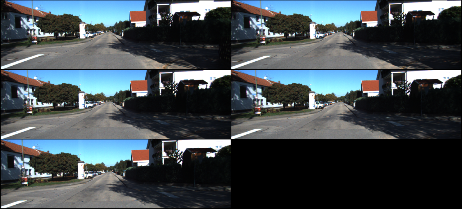
Reversing the image normalisation, we can display the first batch of images from Sequence 5, the test sequence:
import matplotlib.pyplot as plt

from torchvision.utils import make_grid

def show(imgs):
    if not isinstance(imgs, list):
        imgs = [imgs]
    fig, axs = plt.subplots(ncols=len(imgs), squeeze=False)
    for i, img in enumerate(imgs):
        img = img.detach()
        img = TF.to_pil_image(img)
        axs[0, i].imshow(np.asarray(img))
        axs[0, i].set(xticklabels=[], yticklabels=[], xticks=[], yticks=[])
    plt.savefig('filename.png', bbox_inches="tight", dpi=300, pad_inches=0)

grid = make_grid(x[0], nrow=2, normalize=True)
show(grid)
Visualizing the Test Trajectory
Now, let’s visualize the test sequence’s trajectory. To achieve this, we must combine the incremental position and orientation data provided in batches and chunks by the dataloader. By systematically accumulating these incremental changes in rotation and translation, we can plot the trajectory. In order to visualise this geographically on a map, we also need to know the latitude and longitude of the origin, as well as the starting yaw angle.
def reconstruct_trajectory(batched_angles, batched_translations, n=5, overlap=1):
    start_angle = [0.0, 0.0, 0.0]
    start_translation = [0.0, 0.0, 0.0]

    # Initialize angle/translation for first batch
    reconstructed_angles = [start_angle]
    reconstructed_translations = [start_translation]

    for i in range(len(batched_translations)):

        # Accumulate angle/translation deltas
        angles = torch.cumsum(batched_angles[i], dim=0)
        translations = torch.cumsum(batched_translations[i], dim=0)

        r0_inv = Tensor(R.from_euler('YXZ', start_angle).as_matrix())
        translations = torch.einsum("ab,cb->ca", r0_inv, translations)

        # Add the last angle/translation to all elements in current batch
        angles += torch.tensor(start_angle)
        translations += torch.tensor(start_translation)

        if i == 0:
            reconstructed_angles.extend(angles.tolist())
            reconstructed_translations.extend(translations.tolist())
        else:
            reconstructed_angles.extend(angles.tolist()[(overlap-n):])
            reconstructed_translations.extend(translations.tolist()[(overlap-n):])

        # Save the angle/translation needed to start the next sequence
        start_angle = reconstructed_angles[-overlap]
        start_translation = reconstructed_translations[-overlap]

    return torch.tensor(reconstructed_translations)
def rotate_points(x, y, angle_degrees):
    """
    Rotate (x, y) points around the origin.

    Parameters:
    - x: array-like, x-coordinates
    - y: array-like, y-coordinates
    - angle_degrees: float, rotation angle in degrees (counterclockwise)

    Returns:
    - x_rotated: array-like, rotated x-coordinates
    - y_rotated: array-like, rotated y-coordinates
    """
    # Convert the rotation angle to radians
    angle_rad = np.radians(angle_degrees)

    # Define the rotation matrix
    rotation_matrix = np.array([
        [np.cos(angle_rad), -np.sin(angle_rad)],
        [np.sin(angle_rad),  np.cos(angle_rad)]
    ])

    # Rotate the points
    xy_rotated = np.dot(rotation_matrix, [x, y])

    return xy_rotated[0], xy_rotated[1]
def local_to_geo(translations, origin_lat, origin_lon, angle_degrees):
    """Convert local coordinates to geographical coordinates."""
    x, y, z = translations.T

    x, z = rotate_points(x, z, angle_degrees)

    R = 6_378_137  # Earth radius in meters
    dlat = z / R
    dlon = x / (R * np.cos(np.pi * origin_lat / 180))

    latitudes = origin_lat + dlat * 180 / np.pi
    longitudes = origin_lon + dlon * 180 / np.pi

    return latitudes, longitudes
import folium


translations = reconstruct_trajectory(y_angles[:, 1:, :], y_translations[:, 1:, :])

# Starting point
origin_lat, origin_lon = 49.049526, 8.396598

# Initial yaw angle
yaw_angle = 10

# Convert local trajectory to geo-coordinates
latitudes, longitudes = local_to_geo(translations, origin_lat, origin_lon, yaw_angle)

m = folium.Map(location=[origin_lat, origin_lon], zoom_start=17)

# Add the trajectory as a polyline
folium.PolyLine(zip(latitudes, longitudes)).add_to(m)

# Display the map
m
Visual Odometry: DeepVO
from torchvision.models.optical_flow import raft_large, Raft_Large_Weights


class Model(pl.LightningModule):
    def __init__(
        self,
        width: int,
        height: int,
        hidden_size: int = 1000,
        dropout=0.5,
        lr: float = 1e-4,
    ):
        super().__init__()
        self.save_hyperparameters()
        self.example_input_array = torch.rand(8, 5, 3, height, width)

        # Freeze pretrained RAFT model
        self.raft = raft_large(weights=Raft_Large_Weights.DEFAULT)
        self.raft.eval()
        for param in self.raft.parameters():
            param.requires_grad = False

        # Define a series of convolutions that increase the channels and reduce the
        # resolution so that RAFT output matches FlowNetSimple output
        self.convs = nn.Sequential(
            nn.Conv2d(2, 64, kernel_size=5, stride=2, padding=2),  # (64, 320, 96)
            nn.ReLU(),
            nn.Conv2d(64, 128, kernel_size=5, stride=2, padding=2),  # (128, 160, 48)
            nn.ReLU(),
            nn.Conv2d(128, 256, kernel_size=5, stride=2, padding=2),  # (256, 80, 24)
            nn.ReLU(),
            nn.Conv2d(256, 512, kernel_size=3, stride=2, padding=1),  # (512, 40, 12)
            nn.ReLU(),
            nn.Conv2d(512, 1024, kernel_size=3, stride=4, padding=1),  # (1024, 10, 3)
            nn.ReLU(),
        )

        input_size = int(np.prod(self.convs(torch.zeros(1, 2, height, width)).size()))

        # RNN
        self.rnn = nn.LSTM(
            input_size=input_size,
            hidden_size=hidden_size,
            num_layers=2,
            batch_first=True,
        )

        self.dropout = nn.Dropout(dropout)
        self.linear_angles = nn.Linear(hidden_size, 3)
        self.linear_translations = nn.Linear(hidden_size, 3)

    def forward(self, x):
        batch_size, seq_len, channel, height, width = x.shape
        flows = self.raft(
            x[:, :-1].reshape(-1, channel, height, width),
            x[:, 1:].reshape(-1, channel, height, width),
        )[-1]
        flows = flows.reshape(batch_size, seq_len - 1, 2, height, width)
        feature_maps = self.convs(flows.reshape(-1, 2, height, width))
        out, _ = self.rnn(feature_maps.reshape(batch_size, seq_len - 1, -1))
        out = self.dropout(out)
        angles = self.linear_angles(out)
        translations = self.linear_translations(out)
        return flows, angles, translations

    def training_step(self, batch, batch_idx):
        loss = self._shared_eval_step(batch, batch_idx)
        self.log(
            "train_loss",
            loss,
            on_step=True,
            on_epoch=True,
            sync_dist=True,
            prog_bar=True,
        )
        return loss

    def validation_step(self, batch, batch_idx):
        loss = self._shared_eval_step(batch, batch_idx)
        metrics = {"val_loss": loss}
        self.log_dict(metrics, sync_dist=True)
        return metrics

    def _shared_eval_step(self, batch, batch_idx):
        x, y_angles, y_translations = batch
        flows, y_hat_angles, y_hat_translations = self(x)
        angle_loss = F.mse_loss(y_hat_angles, y_angles[:, 1:, :])
        translation_loss = F.mse_loss(y_hat_translations, y_translations[:, 1:, :])
        loss = 100 * angle_loss + translation_loss
        return loss

    def predict_step(self, batch, batch_idx, dataloader_idx=0):
        x, y_angles, y_translations = batch
        return self(x)

    def configure_optimizers(self):
        optimizer = optim.Adam(self.parameters(), lr=self.hparams.lr)
        scheduler = optim.lr_scheduler.ReduceLROnPlateau(
            optimizer, patience=3, verbose=True
        )
        return {
            "optimizer": optimizer,
            "lr_scheduler": {"scheduler": scheduler, "monitor": "val_loss"},
        }

model = Model(640, 192)
DeepVO2 is one of the first models to apply end-to-end deep learning to visual odometry. This model first processes an input sequence of images through the feature extraction segment of FlowNet, an optical flow model. It then feeds the extracted features into a Recurrent Neural Network (RNN) to produce sequences that depict the pose of the subject. FlowNet’s feature extractor accepts a pair of consecutive images (stacked to form a 6-channel input of size 192 by 640) and transforms them, increasing the number of feature channels while compressing the spatial dimensions. The end result is a condensed feature map of size (1024, 3, 10).
In our specific approach, we’ve adapted the model by substituting FlowNet with RAFT, another state-of-the-art model for optical flow computation. To maintain compatibility with the RNN’s expected input dimensions, we reverse-engineer the output from RAFT (which produces a flow map of size 2 by 192 by 640) to mimic the refinement stage seen in FlowNet’s architecture.
Optical Flow: RAFT
An optical flow model is a type of vision algorithm used to estimate the motion of objects between two consecutive frames of a video. It determines how much each pixel in one image moves to the next, capturing the motion of objects, surfaces, and edges in a visual scene. Optical flow is used for motion estimation, video stablisation and object tracking.
RAFT (Recurrent All-Pairs Field Transforms), is a more recent and advanced model for optical flow estimation that is included in Torchvision. While FlowNet uses a straightforward convolutional neural network (CNN), RAFT uses a recurrent neural network to iteratively refine its predictions over time.
To learn more about optical flow and to explore RAFT in detail, see this PyTorch tutorial: Optical Flow: Predicting movement with the RAFT model3
Within our own model, we have designed it to output an intermediate representation of the optical flow. This allows us to visually examine the flow patterns that RAFT detects and interprets.
trainer = pl.Trainer(limit_predict_batches=1, accelerator="gpu", devices=1)
output = trainer.predict(model=model, datamodule=datamodule)
flows, _, _ = tuple(map(torch.cat, zip(*output)))
GPU available: True (cuda), used: True
TPU available: False, using: 0 TPU cores
IPU available: False, using: 0 IPUs
HPU available: False, using: 0 HPUs
/home/timothy/dev/blog/.venv/lib/python3.9/site-packages/lightning/pytorch/trainer/connectors/logger_connector/logger_connector.py:67: UserWarning: Starting from v1.9.0, `tensorboardX` has been removed as a dependency of the `lightning.pytorch` package, due to potential conflicts with other packages in the ML ecosystem. For this reason, `logger=True` will use `CSVLogger` as the default logger, unless the `tensorboard` or `tensorboardX` packages are found. Please `pip install lightning[extra]` or one of them to enable TensorBoard support by default
  warning_cache.warn(
`Trainer(limit_predict_batches=1)` was configured so 1 batch will be used.
LOCAL_RANK: 0 - CUDA_VISIBLE_DEVICES: [0,1]


Predicting DataLoader 0: 100%|████████████████████| 1/1 [00:01<00:00,  1.33s/it]
Using the code from the blog post, we plot a single batch of input images and optical flows:
from torchvision.utils import flow_to_image

flow_imgs = [img/255 for img in flow_to_image(flows[0])]
imgs = [(img + 1) / 2 for img in x[0]]
grid = make_grid([img for pair in zip(imgs, flow_imgs) for img in pair], nrow=2)
show(grid)
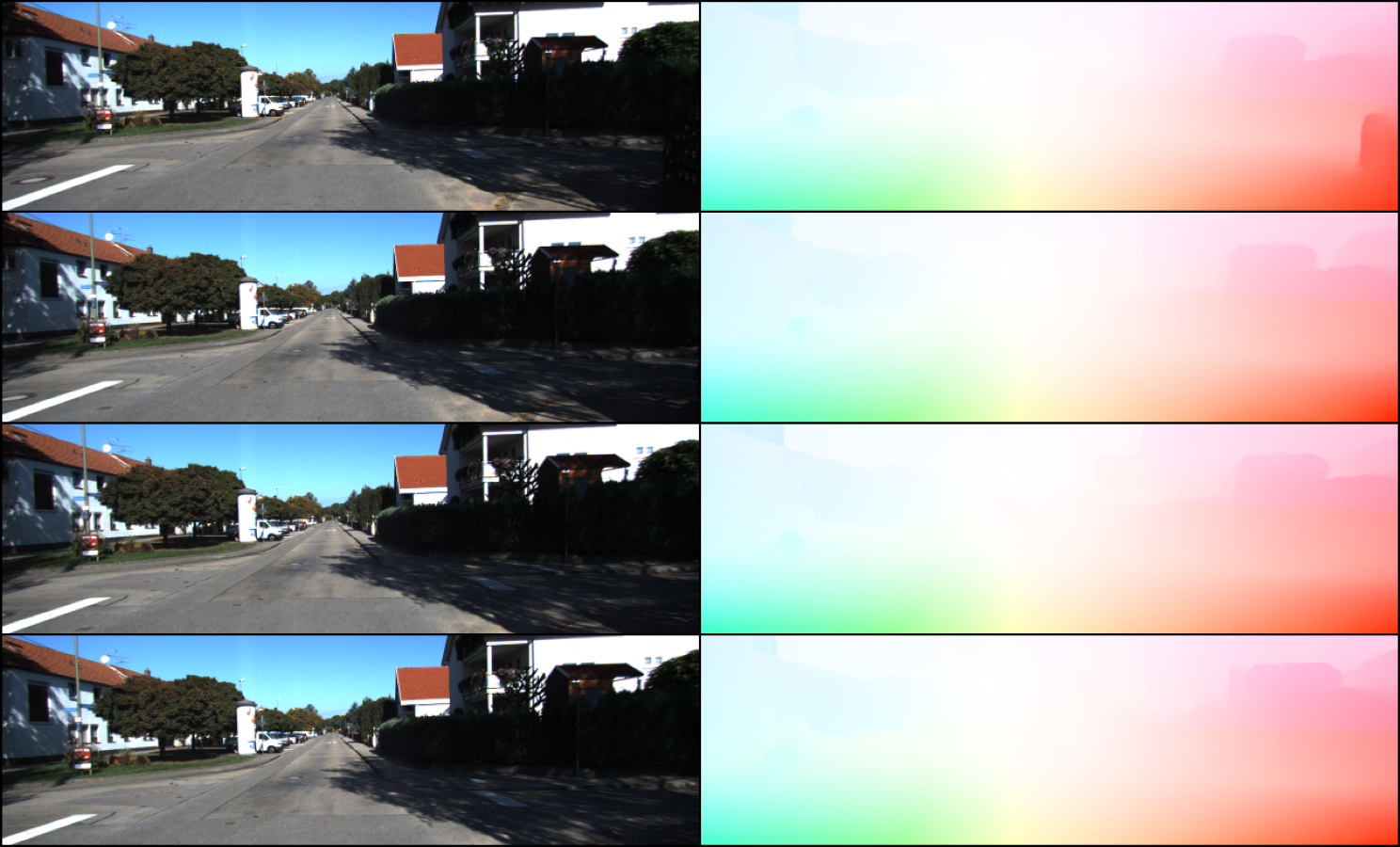
Note: since the car is moving forwards, the pixels move outwards away from the center vanishing point, meaning that the pixels on the left move further left and the pixels on the right move further right.
Model Training
from lightning.pytorch.callbacks.early_stopping import EarlyStopping
from lightning.pytorch.callbacks.model_summary import ModelSummary


wandb_logger = pl.loggers.WandbLogger()
early_stopping = EarlyStopping(monitor="val_loss", patience=6, verbose=True)
model_summary = ModelSummary(max_depth=2)

trainer = pl.Trainer(
    max_epochs=-1,
    logger=wandb_logger,
    callbacks=[early_stopping, model_summary],
    accelerator="gpu",
    devices=2,
)
trainer.fit(model=model, datamodule=datamodule)
Using 2 × NVIDIA Quadro GP100, the model takes 5 hours to train.
Reconstructing the Predicted Trajectory
In the same way that we reconstructed the trajectory from the input data, we can do the same with the predicted angle and translation deltas.
trainer = pl.Trainer(accelerator="gpu", devices=1)
output = trainer.predict(model=model, datamodule=datamodule)
flows, y_hat_angles, y_hat_translations = tuple(map(torch.cat, zip(*output)))
# Reconstruct predicted trajectory from predicted angle and translation deltas
translations = reconstruct_trajectory(y_hat_angles, y_hat_translations)

# Convert local predicted trajectory to geo-coordinates
latitudes, longitudes = local_to_geo(translations, origin_lat, origin_lon, 10)

# Add the predicted trajectory as a polyline
folium.PolyLine(zip(latitudes, longitudes), color="red").add_to(m)

# Display the map
m
Note: as the predicted trajectory progresses, the discrepancy from the actual ground truth increases due to the accumulation of errors.
References
-
Geiger, A., Lenz, P. & Urtasun, R. (2012). Are we ready for Autonomous Driving? The KITTI Vision Benchmark Suite. Conference on Computer Vision and Pattern Recognition (CVPR). ↩︎
-
Wang, S., Clark, R., Wen, H. K., & Trigoni, N. (2017). DeepVO: Towards End-to-End Visual Odometry with Deep Recurrent Convolutional Neural Networks. International Conference on Robotics and Automation (ICRA). ↩︎
-
Hug, N., Oke, A. & Vryniotis, V. (2022). Optical Flow: Predicting movement with the RAFT model. Torchvision documentation. ↩︎
Timothy Leung, Markus Burki